Decision trees are a popular machine learning algorithm that can be used for both classification and regression tasks. They are easy to understand and interpret, and they can handle both numerical and categorical data. Moreover, some more advanced algorithms are based on decision trees, such as Random Forests and Gradient Boosting.
Let’s illustrate the concept with a classification example.
11.1 Decision Trees for Classification
We will use the (in)famous Iris dataset, which contains information about three different species of iris flowers. The goal is to classify the species based on the sepal length, sepal width, petal length, and petal width of the flowers. Table 11.1 shows a preview with a few first rows from the dataset.
Code
# Load the Iris datasetfrom sklearn.datasets import load_irisiris = load_iris()# Create a DataFrame with the feature variablesimport pandas as pddata = pd.DataFrame(iris.data, columns=iris.feature_names)# Add the target variable to the DataFramedata['species'] = iris.target# Display the first few rows of the DataFramedata.head()
Table 11.1: First few rows of the Iris dataset
sepal length (cm)
sepal width (cm)
petal length (cm)
petal width (cm)
species
0
5.1
3.5
1.4
0.2
0
1
4.9
3.0
1.4
0.2
0
2
4.7
3.2
1.3
0.2
0
3
4.6
3.1
1.5
0.2
0
4
5.0
3.6
1.4
0.2
0
Now let’s say we would want to predict the species of an iris flower based on its sepal length and sepal width. We can train a decision tree classifier on the data and visualize the decision boundaries.
11.1.1 Building a Decision Tree Classifier
We can fit a decision tree to our data with the help of scikit-learn. The first step, as always, is to select the feature variables and split the data into training and testing sets.
# Load the necessary librariesfrom sklearn import treefrom sklearn.model_selection import train_test_split# Select the feature variablesX = data[['sepal length (cm)', 'sepal width (cm)']]y = data['species']# Split the data into training and testing setsX_train, X_test, y_train, y_test = train_test_split(X, y, test_size=0.25, random_state=42)# Create a decision tree classifiertree_classifier = tree.DecisionTreeClassifier(max_depth=3)# Train the classifier on the training datatree_classifier.fit(X_train, y_train)
DecisionTreeClassifier(max_depth=3)
In a Jupyter environment, please rerun this cell to show the HTML representation or trust the notebook. On GitHub, the HTML representation is unable to render, please try loading this page with nbviewer.org.
DecisionTreeClassifier(max_depth=3)
Above we used the tree module from scikit-learn to create a decision tree classifier with a maximum depth of 3. We will see in a moment what this means. The classifier is then trained on the training data. We left 25% of the data as our test set. The predict method allows us to, well, predict the species of the flowers in the test set:
# Make predictions on the test datay_pred = tree_classifier.predict(X_test)print(y_pred)
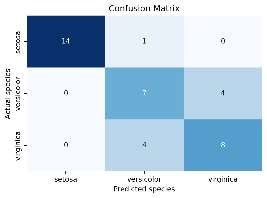
The test predictions above are stored in a variable y_pred. We can now evaluate the model’s performance by computing the confusion matrix. Figure 11.1 shows the confusion matrix for the decision tree classifier.
Code
# Load the necessary librariesfrom sklearn.metrics import confusion_matriximport seaborn as snsimport matplotlib.pyplot as plt# Compute the confusion matrixcm = confusion_matrix(y_test, y_pred)plt.figure(figsize=(6, 4))sns.heatmap(cm, annot=True, fmt='d', cmap='Blues', cbar=False, xticklabels=iris.target_names, yticklabels=iris.target_names)plt.xlabel('Predicted species')plt.ylabel('Actual species')plt.title('Confusion Matrix')plt.show()
Figure 11.1: Confusion matrix showing the performance of the decision tree classifier on the test data.
We can tell by looking at the confusion matrix that the model seems quite capable of distinguishing between the three species of iris flowers. But how does it actually achieve this? Let’s visualize the decision making process.
11.1.2 Visualizing the Decision Boundaries
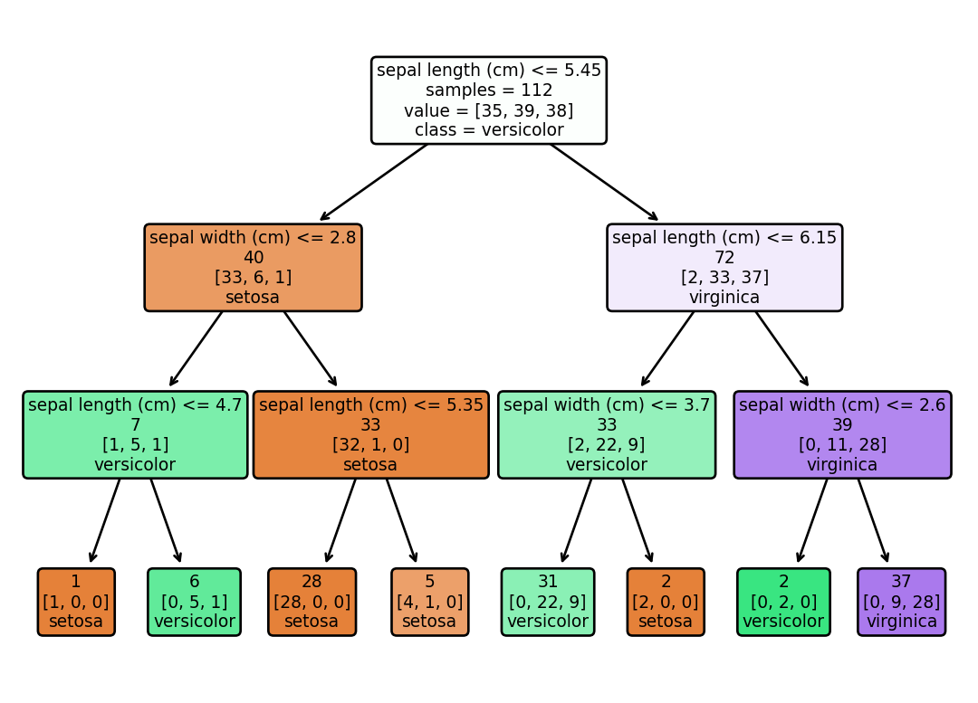
Decision trees are called so due to the visual appearance of the model. The tree consist of nodes that represent decisions based on the input features. We can visualize the nodes an splits in the data with the plot_tree function from the sklearn.tree module. Figure 11.2 shows the decision boundaries of the trained decision tree classifier.
Figure 11.2: The visualization of the decision tree shows how the classification predictions are made based on the input features. Each node represents a decision based on a feature, and the color represents the predicted class.
Visualizing the decision boundaries can help us understand how the decision tree classifier makes predictions based on the input features. For example, from the Figure 11.2 we can see that the classifier first checks if the sepal length is less than 5.45 cm. If it is, the flower is classified as setosa. Observations where sepal length is equal to or above 5.45 cm are classified as virginica. Similar decisions are made twice more, which corresponds to the max_depth=3 parameter we set when creating the classifier. This decision making process categorizes our data into three distinct classes. But how is the algorithm able to make these decisions?
11.2 Decision Trees for Regression
Decision trees can be applied to regression problems as well. Our workflow will be almost analogous to the one we used for classification. We will use the California housing dataset, which contains information about various features of houses in California and their corresponding prices. The goal is to predict the price of a house based on its features. Table 11.2 shows a preview with a few first rows from the dataset.
Code
# Load the California housing datasetfrom sklearn.datasets import fetch_california_housingcalifornia_housing = fetch_california_housing()data = pd.DataFrame(california_housing.data, columns=california_housing.feature_names)data['MedVal'] = california_housing.targetdata.head()
Table 11.2: First few rows of the California housing dataset
MedInc
HouseAge
AveRooms
AveBedrms
Population
AveOccup
Latitude
Longitude
MedVal
0
8.3252
41.0
6.984127
1.023810
322.0
2.555556
37.88
-122.23
4.526
1
8.3014
21.0
6.238137
0.971880
2401.0
2.109842
37.86
-122.22
3.585
2
7.2574
52.0
8.288136
1.073446
496.0
2.802260
37.85
-122.24
3.521
3
5.6431
52.0
5.817352
1.073059
558.0
2.547945
37.85
-122.25
3.413
4
3.8462
52.0
6.281853
1.081081
565.0
2.181467
37.85
-122.25
3.422
The data contains information about various features of houses in California. Let’s take a looks at the description of the dataset to understand what each feature represents.
Code
print(california_housing.DESCR)
.. _california_housing_dataset:

California Housing dataset
--------------------------

**Data Set Characteristics:**

    :Number of Instances: 20640

    :Number of Attributes: 8 numeric, predictive attributes and the target

    :Attribute Information:
        - MedInc        median income in block group
        - HouseAge      median house age in block group
        - AveRooms      average number of rooms per household
        - AveBedrms     average number of bedrooms per household
        - Population    block group population
        - AveOccup      average number of household members
        - Latitude      block group latitude
        - Longitude     block group longitude

    :Missing Attribute Values: None

This dataset was obtained from the StatLib repository.
https://www.dcc.fc.up.pt/~ltorgo/Regression/cal_housing.html

The target variable is the median house value for California districts,
expressed in hundreds of thousands of dollars ($100,000).

This dataset was derived from the 1990 U.S. census, using one row per census
block group. A block group is the smallest geographical unit for which the U.S.
Census Bureau publishes sample data (a block group typically has a population
of 600 to 3,000 people).

A household is a group of people residing within a home. Since the average
number of rooms and bedrooms in this dataset are provided per household, these
columns may take surprisingly large values for block groups with few households
and many empty houses, such as vacation resorts.

It can be downloaded/loaded using the
:func:`sklearn.datasets.fetch_california_housing` function.

.. topic:: References

    - Pace, R. Kelley and Ronald Barry, Sparse Spatial Autoregressions,
      Statistics and Probability Letters, 33 (1997) 291-297
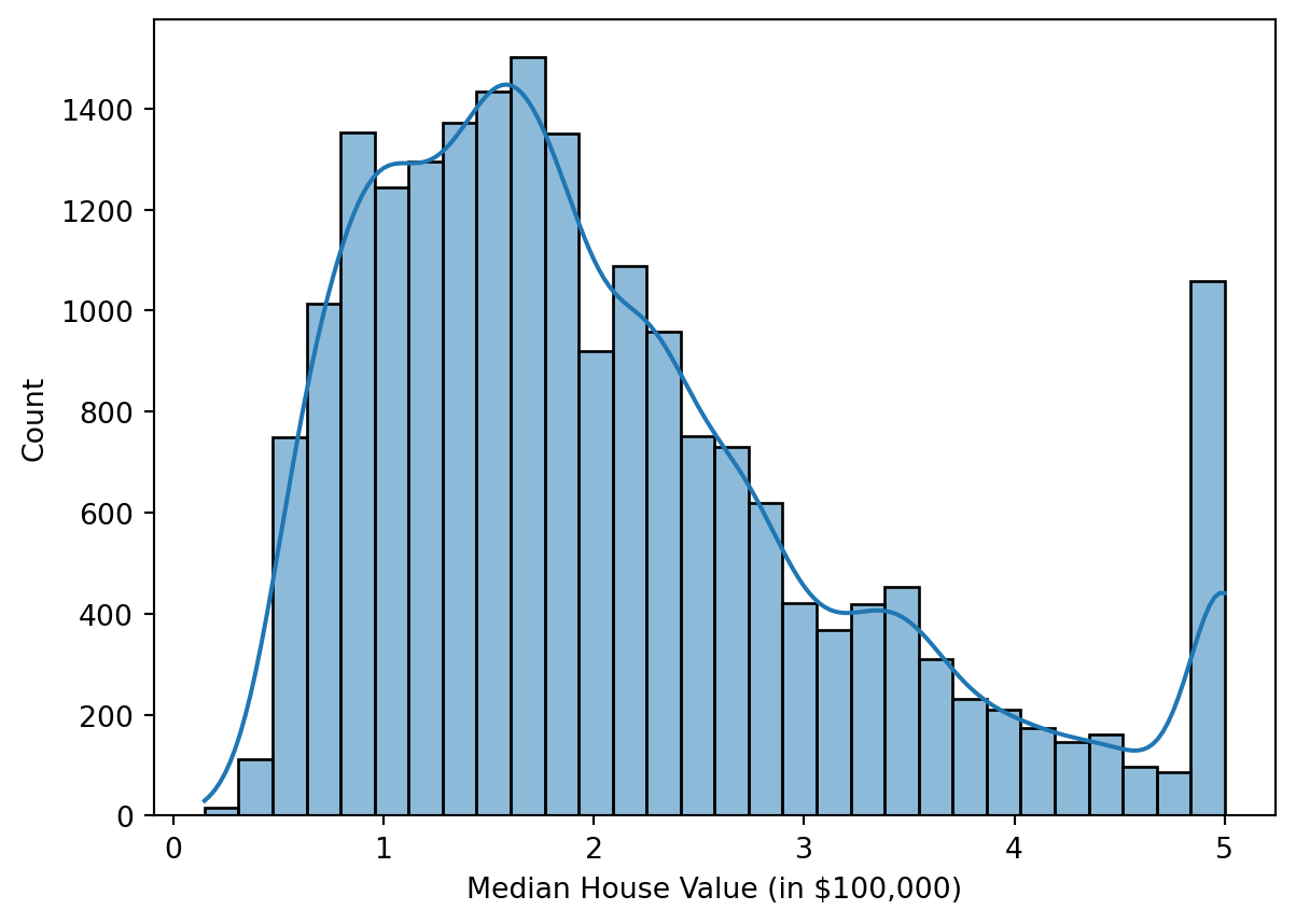
The description gives us a pretty thorough overview of what we are dealing with. The MedVal column is what we are trying to predict, and it represents the median value of a house in California in units of $100,000. Figure 11.3 shows the distribution of the median house values in the dataset.
Code
x = sns.histplot(data['MedVal'], bins=30, kde=True)x.set_xlabel('Median House Value (in $100,000)')# show the plotplt.show()
Figure 11.3: Histogram showing the distribution of the median house values in the California housing dataset.
The distribution seems to have a Poisson-like shape, with a long tail on the right. The only thing that sticks out is the bar around $500,000, which might indicate that the prices are capped at that value. For now we will ignore this and proceed with the regression task.
Code
X = california_housing.datay = california_housing.targetX_train, X_test, y_train, y_test = train_test_split(X, y,test_size=0.25, random_state=42)# Create a decision tree regressorfrom sklearn.tree import DecisionTreeRegressortree_regressor = DecisionTreeRegressor(max_depth=3)# Train the regressor on the training datatree_regressor.fit(X_train, y_train)# Make predictions on the test datay_pred = tree_regressor.predict(X_test)# Compute the mean squared errorfrom sklearn.metrics import mean_squared_errormse = mean_squared_error(y_test, y_pred)print(f'Mean Squared Error: {mse:.2f}')
Mean Squared Error: 0.64
11.3 How Decision Trees Work
WIP…
The Gini index is a measure of impurity used by the decision tree algorithm to determine the best split at each node. The Gini index is calculated as follows:
\[
G = 1 - \sum_{i=1}^{n} p_i^2
\]
where \(p_i\) is the probability of observing class \(i\) in a given node. The Gini index ranges from 0 to 1, where 0 indicates that the node is pure (i.e., all observations belong to the same class) and 1 indicates that the node is impure (i.e., observations are evenly distributed among classes).
Entropy is another measure of impurity that can be used by the decision tree algorithm. The entropy of a node is calculated as follows:
\[
H = -\sum_{i=1}^{n} p_i \log_2(p_i)
\]
where \(p_i\) is the probability of observing class \(i\) in a given node. The entropy ranges from 0 to \(\log_2(n)\), where 0 indicates that the node is pure (i.e., all observations belong to the same class) and \(\log_2(n)\) indicates that the node is impure (i.e., observations are evenly distributed among classes).