9  Linear regression

Linear regression is fancy way of describing the act of fitting a line through your data. What makes it powerful is it’s simplicity. When we are facing a regression problem this is usually the first thing we should try before moving on to more complex models. If you are looking for a detailed explanation on the intricacies of linear regression, I recommend taking a closer look at the wonderful book by James, Witten, Hastie and Tibshirani titled An Introduction to Statistical Learning (James et al. (2023)).

Regression in a nutshell

In regression we are trying to predict a numerical (continuous) variable based on one or more other variables. The variable we are trying to predict is called the dependent variable, and the variables we are using to make the prediction are called the independent variables. In the field of Data Science, the dependent variable can sometimes be called the outcome, and the independent variables might be referred to as features.

9.1 Simple linear regression

Simple linear regression is the most basic form of regression. It is used when we want to use the values of a single independent variable to predict the values for the dependent variable. To put it simply, the goal is to find the best-fitting straight line through the data. The equation for a simple linear regression model is:

\[ y = \beta_0 + \beta_1x \text{,} \tag{9.1}\]

where \(y\) is the dependent variable, \(x\) is the independent variable, \(\beta_0\) is the intercept, \(\beta_1\) is the slope.

Let’s see how we can implement simple linear regression in Python using the scikit-learn library. Scikit-learn is one of the most fundamental machine learning libraries for Python. It provides a wide range of tools for building machine learning models, including regression models. Before we start, we need to install the library. You can do this by running the following command in your terminal:

pip install scikit-learn

After installation, we are ready to implement a simple linear regression model. We will use data from the World Happiness Report 2019, which is available through Kaggle (Kaggle Datasets (2024)). The World Happiness Report is a survey of the state of global happiness that ranks 156 countries by how happy their citizens perceive themselves to be. The dataset contains information about various factors that contribute to happiness, such as GDP per capita, social support, healthy life expectancy, freedom to make life choices, generosity, and perceptions of corruption (Table 9.1).

import pandas as pd
import seaborn as sns

# get the diamonds dataset
happiness = pd.read_csv('data/WorldHappinessReport2019.csv')
happiness.head()

Table 9.1: The first rows of the World Happiness Report 2019 dataset.

	Overall rank	Country or region	Score	GDP per capita	Social support	Healthy life expectancy	Freedom to make life choices	Generosity	Perceptions of corruption
0	1	Finland	7.769	1.340	1.587	0.986	0.596	0.153	0.393
1	2	Denmark	7.600	1.383	1.573	0.996	0.592	0.252	0.410
2	3	Norway	7.554	1.488	1.582	1.028	0.603	0.271	0.341
3	4	Iceland	7.494	1.380	1.624	1.026	0.591	0.354	0.118
4	5	Netherlands	7.488	1.396	1.522	0.999	0.557	0.322	0.298

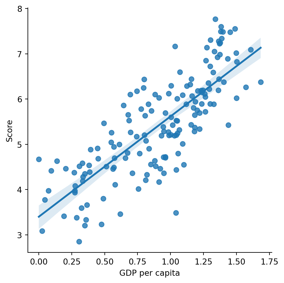
Figure 9.1 visualizes the relationship between a country’s happiness Score and GDP per capita. We can see that, on average countries with higher GDP per capita exhibit higher levels of happiness.

sns.lmplot(x='GDP per capita', y='Score', data=happiness)

Figure 9.1: A scatter plot showing the relationship between the happiness score and the GDP per capita. Note that correlation does not imply causation.

9.1.1 Fitting the model with scikit-learn

Above we used our seaborn knowledge to visualize the linear relationship. However, this doesn’t actually give as a model with stored parameter values. In order to actually fit the model shown in Equation 9.1, we can use LinearRegression from scikit-learn.

from sklearn.linear_model import LinearRegression

# create a linear regression model object
model = LinearRegression()

# fit the model to the data
model.fit(X=happiness[['GDP per capita']], y=happiness['Score'])

# print the model coefficients
model.coef_, model.intercept_

(array([2.218148]), 3.399345178292417)

Let’s go throught the code above line by line. First, we import the LinearRegression Estimator from the sklearn.linear_model family of models. Next, we create a LinearRegression object called model. We then fit the model to the data using the fit method. The fit method takes two arguments: the independent variable X and the dependent variable y. In this case, we are using GDP per capita as the independent variable and Score as the dependent variable. Finally, we print the model coefficients. The coef_ attribute contains the slope of the line, and the intercept_ attribute contains the intercept.

Let’s now look at Figure 9.1 again, to help us understand the model we just fitted. The slope of the line is the coefficient for GDP per capita (\(\beta_1\) in Equation 9.1), and the intercept is the value of the dependent variable when GDP per capita is zero. In other words, the intercept is the y-value where the fitted line crosses the y-axis. By looking at the plot, we can see that the intercept is around 3.4, which is the result we got from our fitted model as well. The slope is around 2.2, which means that for every unit increase in GDP per capita, the Score increases by 2.2 units. This is the beauty of linear regression - it gives us a simple and interpretable model that we can use to make predictions.

9.1.2 Making predictions

Now that we have a fit for our model to the data, we can use it to make predictions. In this case the model is very simple, so we could easily calculate the predictions by hand as well. Let’s predict the happiness score for the countries in the dataset. The results for the first five entries are displayed in Table 9.2.

# make a prediction for all the countries in the dataset
X_new = happiness[['GDP per capita']]
preds = model.predict(X_new)

## create a dataframe with the predictions, GDP per capita and the actual score
preds_df = pd.DataFrame({
    'GDP per capita': X_new['GDP per capita'],
    'Predicted score': preds,
    'Actual score': happiness['Score']
})

preds_df.head()

Table 9.2: The actual happiness score and the predicted score based on the GDP per capita.

	GDP per capita	Predicted score	Actual score
0	1.340	6.371663	7.769
1	1.383	6.467044	7.600
2	1.488	6.699949	7.554
3	1.380	6.460389	7.494
4	1.396	6.495880	7.488

The GDP per capita value for the first entry is 1.34. Let’s calculate the predicted score “by hand” using the model coefficients:

# calculate the predicted score for the first entry
predicted_score = model.intercept_ + model.coef_[0] * 1.34
predicted_score

6.371663499643615

Lo and behold, we get the same result as by using the predict method (as we should).

9.1.3 Evaluating model performance

Now that we have our predictions, we are ready to evaluate how successful we were with the fitting process. There are different ways to evaluate the performance of a regression model, but we are going to look at three commonly used metrics. Namely:

• Mean Squared Error (MSE)
• Root Mean Squared Error (RMSE)
• Mean Absolute Error (MAE).

MSE in defined as follows:

\[ \text{MSE} = \frac{1}{n} \sum_{i=1}^{n} (y_i - \hat{y}_i)^2 \text{,} \]

where \(y_i\) is the actual value for the \(i\)th observation, \(\hat{y}_i\) is the corresponding predicted value, and \(n\) is the number of observations. So basically we are just looking at the average of the squared differences between the actual and predicted values. RMSE is simply the square root of the MSE:

\[ \text{RMSE} = \sqrt{\frac{1}{n} \sum_{i=1}^{n} (y_i - \hat{y}_i)^2} \text{.} \]

MAE is possibly the most intuitive of the three, as it is simply the average of the absolute differences between the actual and predicted values:

\[ \text{MAE} = \frac{1}{n} \sum_{i=1}^{n} |y_i - \hat{y}_i| \text{.} \]

We can now calculate these metrics for our model. Let’s add squared and absolute differences to the predictions dataframe and calculate the metrics. Table 9.3 shows the head of the updated dataframe.

# calculate the squared and absolute differences
preds_df['Sqr. diff'] = (preds_df['Actual score'] - preds_df['Predicted score'])**2
preds_df['Abs. diff'] = abs(preds_df['Actual score'] - preds_df['Predicted score'])

preds_df.head()

Table 9.3: The squared and absolute differences between the actual and predicted scores for the first five entries.

	GDP per capita	Predicted score	Actual score	Sqr. diff	Abs. diff
0	1.340	6.371663	7.769	1.952549	1.397337
1	1.383	6.467044	7.600	1.283590	1.132956
2	1.488	6.699949	7.554	0.729402	0.854051
3	1.380	6.460389	7.494	1.068351	1.033611
4	1.396	6.495880	7.488	0.984303	0.992120

We can now calculate the MSE, RMSE, and MAE for the model.

MSE = preds_df['Sqr. diff'].mean()
RMSE = MSE**0.5
MAE = preds_df['Abs. diff'].mean()

MSE, RMSE, MAE

(0.4551967397324354, 0.6746826955928508, 0.5490499282630026)

Scikit-learn also provides a convenient way to calculate these metrics using the mean_squared_error and mean_absolute_error functions from the sklearn.metrics module. Let’s see if we get the same results using these functions.

from sklearn.metrics import mean_squared_error, mean_absolute_error

MSE = mean_squared_error(happiness['Score'], preds)
RMSE = mean_squared_error(happiness['Score'], preds, squared=False)
MAE = mean_absolute_error(happiness['Score'], preds)

MSE, RMSE, MAE

(0.4551967397324354, 0.6746826955928508, 0.5490499282630026)

Phew, what a relief! The results are the same as with our manual calculation. These convenient functions are actually the one’s we’ll be using from now on.

We have now successfully fitted a simple linear regression model to the data, made predictions, and evaluated the model’s performance. Unfortunately, as it turns out, we have taken some shortcuts in the process which we need to address.

Warning

You should never use all you data to fit a model. The reason is that the model will be biased towards the data it has seen, and has a higher probability of not generalizing well to new data. There is a large risk of something called overfitting, which we will learn more about in the next section.

9.2 Re-fitting the model the proper way

In the previous example, we used only one feature to predict the happiness score. However, oftentimes we want to use multiple features to make the prediction. This is called multiple linear regression. The equation for multiple linear regression is:

\[ y = \beta_0 + \sum_{i=1}^{n} \beta_i x_i \text{,} \tag{9.2}\]

where \(y\) is the dependent variable, \(x_1, x_2, \ldots, x_n\) are the independent variables, \(\beta_0\) is the intercept, and \(\beta_1, \beta_2, \ldots, \beta_n\) are the coefficients for each independent variable.

Now, there is actually nothing wrong with using only a single feature to predict the happiness score. However, as we discussed above, you shouldn’t use all your data to fit the model. Instead, you should split the data into training and test sets, and fit the model using only the training data. We’ll learn more about this next.

9.2.1 The train-test split

Splitting the data into training and test sets is a crucial step in the machine learning workflow. It is such a standard procedure that scikit-learn comes with a built in function to help us get the job done. This is important because we want to evaluate the model on data that it hasn’t seen before. This helps prevent overfitting, and let’s us see how well the model performs on new data. However, before we are ready to split the data into training and test sets, we first need to decide which features to use in our model. This usually means dividing the data into features (X) and the target variable (y). We’ll use all the numeric columns except the Score column as features, and the Score column as the target variable.

X = happiness[['GDP per capita', 'Social support', 'Healthy life expectancy', 
'Freedom to make life choices', 'Generosity', 
'Perceptions of corruption']]
y = happiness['Score']

Now that our data is setup correctly, we can split it into training and test sets. To do this, we use the train_test_split function from scikit-learn.

from sklearn.model_selection import train_test_split

X_train, X_test, y_train, y_test = train_test_split(
    X, y, test_size=0.20, random_state=123
    )

Above we passed the X and y dataframes to the train_test_split function. The test_size parameter specifies the proportion of the data that should be used for the test set. In this case, we used 20% of the data for the test set. The random_state parameter is used to ensure that the split is reproducible. By setting the random state to a fixed value, we get the same “random” split every time we run the code.

Before fitting the model, let’s take a look at the shape of the training and test sets.

X_train.shape, X_test.shape, y_train.shape, y_test.shape

((124, 6), (32, 6), (124,), (32,))

We can see that the training set contains 124 observations and the test set contains 32 observations. So roughly 80% of the data is used for training and 20% for testing, just as we requested.

We are now ready to fit the model using the training data.

model2 = LinearRegression()

# fit the model to the training data
model2.fit(X_train, y_train)

# save the model coefficients and intercept to a dataframe
coefficients = pd.DataFrame({
    'feature': ['Intercept'] + X.columns.tolist(),
    # intercept and coefficients
    'value': [model2.intercept_] + model2.coef_.tolist()
})

Here we only used the training data to fit the model. This means that the model has never seen the test data before, and we can use it for getting an unbiased estimate of the model’s performance. Table 9.4 shows the coefficients for each feature in the fitted linear regression model.

Table 9.4: The intercept and coefficient values for each feature in the fitted linear regression model.

	feature	value
0	Intercept	1.668718
1	GDP per capita	0.864532
2	Social support	1.038075
3	Healthy life expectancy	1.113857
4	Freedom to make life choices	1.651626
5	Generosity	0.982648
6	Perceptions of corruption	0.853486

9.2.2 Evaluating the model

Let’s now evaluate our second model using the test data and the metrics we discussed earlier. In order to do this, we need to first make predictions with our test data.

# make predictions on the test data
y_pred = model2.predict(X_test)

# calculate the MSE, RMSE, and MAE
MSE = mean_squared_error(y_test, y_pred)
RMSE = mean_squared_error(y_test, y_pred, squared=False)
MAE = mean_absolute_error(y_test, y_pred)

MSE, RMSE, MAE

(0.3104436244813814, 0.5571746804022787, 0.43781582428696403)

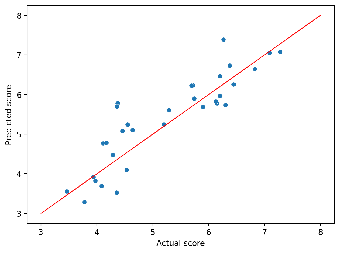
These metrics give us an idea of how well the model is performing. The lower the values, the better the model. Generally, there is a distinction between the training and test error. The numbers above show the test error, which is the most important one as it gives us an indication of how well the model performs on unseen data. Unfortunately, the numerical metrics shown above aren’t always that easy to interpret, which is why visualizations can be helpful. Figure 9.2 shows the actual and predicted happiness scores for the test data. In this case we see that our predictions are fairly well in line with the actual scores.

import matplotlib.pyplot as plt

plot = sns.scatterplot(x=y_test, y=y_pred)
# add axis labels
plot.set_xlabel('Actual score')
plot.set_ylabel('Predicted score')
# add a diagonal line
plt.plot([3, 8], [3, 8], color='red', linewidth=1)

plt.show()

Figure 9.2: A scatter plot showing the actual and predicted happiness scores for the test data. For a perfect prediction all the points would be lined up in a straight line (with a slope of 1).

The linear regression is a fairly rigid method in terms of how well it can accommodate to the training data, which means that the risk of overfitting is not as high as with more complex and flexible models. However, it is important to learn to use the train-test split every time you fit a model, regardless of the model complexity.

Bias-variance trade-off

When discussing model performance, it is important to understand the concept of the bias-variance trade-off. Bias refers to the error that is introduced by approximating a possibly complex real-world problem, with a simple model such as linear regression. Variance, on the other hand, refers to the error that is introduced by using a model that can accommodate the random noise in the data. If we are using a very flexible model, such as a deep neural network, our model coefficients might change a lot depending on the training data. Ideally we would not want this to happen, as it might mean that our model is not generalizing well to new data. The idea of the test-train split is to help us avoid overfitting our model to the training data. For a more in-depth discussion on the bias-variance trade-off, I recommend the book by James et al. (James et al. (2023)).

Now we have the metrics, and we have the estimates for our model coefficients. What if we want to know how confident we can be with these estimates? What if we want to know which features are the most important for predicting the happiness score? For this we need to have an idea of the statistical significance of the coefficients.

9.3 Re-fitting our model with statsmodels

scikit-learn is a great library for building machine learning models, but in case of linear regression it doesn’t provide a way to readily evaluate the statistical significance of the coefficients. For this we can use a Python module called statsmodels. You should already be familiar how to install new libraries by now, so let’s see how we can use statsmodels to fit a linear regression model.

import statsmodels.api as sm

# add a constant to the features
X_train = sm.add_constant(X_train)

# create a linear regression model
model3 = sm.OLS(y_train, X_train)
results = model3.fit()

# print the summary of the model
print(results.summary())

                            OLS Regression Results                            
==============================================================================
Dep. Variable:                  Score   R-squared:                       0.784
Model:                            OLS   Adj. R-squared:                  0.773
Method:                 Least Squares   F-statistic:                     70.73
Date:                Sat, 23 Nov 2024   Prob (F-statistic):           1.33e-36
Time:                        19:08:33   Log-Likelihood:                -94.331
No. Observations:                 124   AIC:                             202.7
Df Residuals:                     117   BIC:                             222.4
Df Model:                           6                                         
Covariance Type:            nonrobust                                         
================================================================================================
                                   coef    std err          t      P>|t|      [0.025      0.975]
------------------------------------------------------------------------------------------------
const                            1.6687      0.238      7.000      0.000       1.197       2.141
GDP per capita                   0.8645      0.253      3.412      0.001       0.363       1.366
Social support                   1.0381      0.267      3.882      0.000       0.509       1.568
Healthy life expectancy          1.1139      0.368      3.028      0.003       0.385       1.842
Freedom to make life choices     1.6516      0.419      3.938      0.000       0.821       2.482
Generosity                       0.9826      0.569      1.725      0.087      -0.145       2.110
Perceptions of corruption        0.8535      0.594      1.438      0.153      -0.322       2.029
==============================================================================
Omnibus:                        8.281   Durbin-Watson:                   1.968
Prob(Omnibus):                  0.016   Jarque-Bera (JB):                8.287
Skew:                          -0.513   Prob(JB):                       0.0159
Kurtosis:                       3.742   Cond. No.                         28.0
==============================================================================

Notes:
[1] Standard Errors assume that the covariance matrix of the errors is correctly specified.

We used the same X_train data as before, but this time we added a constant to the features (this is something that statsmodels needs for fitting the intercept). We then created an OLS (Ordinary Least Squares) model object and fit it to the training data. Finally, we printed the summary of the model.

As a printout we get a lot of stuff. Most importantly, however, we can see that the coefficient values are the same as with scikit-learn. Moreover, we now have 95% confidence intervals for the coefficients, as well as p-values for testing the null hypothesis that the coefficient is equal to zero.

9.4 Conclusion

In this chapter we learned about linear regression, which is a simple yet powerful method for regression analysis. In the next chapter we will get our feet wet with classification, which is also a type of supervised learning problem where the goal is to predict the class of an observation based on the values of the independent variables. We will be using logistic regression, which is a classification algorithm that is closely related to linear regression.

Supervised learning

Supervised learning is a concept in machine learning where our data contains the correct answers. This means that we have a dataset where we know the values of the dependent variable for each observation. The goal of supervised learning is to connect these correct answers to the predictors, so that we can make predictions on new data. Regression and classification are two types of supervised learning problems. There is also unsupervised learning, which we will learn more about later.

James, Gareth, Daniela Witten, Trevor Hastie, and Robert Tibshirani. 2023. An Introduction to Statistical Learning with Applications in Python. Springer. https://www.statlearning.com/.

Kaggle Datasets. 2024. “World Happiness Report - Dataset.” https://www.kaggle.com/datasets/unsdsn/world-happiness?select=2019.csv.